photos, graphics and article by Capt. Gunter Schütze
In the first part of my contribution about GPS, I wrote about the structure, the functionality, technical and physical basics of GPS:
To GPS (Part 1)
In my announced sequel, the second part of GPS, it is primarily about the technical and physical operational and functional limitations to which GPS is subject. These limitations, in part, have serious implications for the accuracy of GPS, and even go as far as limiting the functionality of GPS in its functions or even making it impossible. In doing so, I anticipate that these are errors that occur on a purely technical or physical basis. Much of these errors are taken into account in the configuration of GPS and implemented by means of appropriate correction tools, in GPS, so that unnoticed by the user, these errors are automatically corrected. But not all errors that occur can be solved by these tools. As a result, the GPS partially or temporarily limited in its functionality or temporarily even not effectively usable.
These bugs have nothing to do with SPOOFING/JAMMING. They are based on functional technical and physical causes, without human action. I will write more about spoofing/jamming at the following and last 3rd Part of GPS about artificial human initiated technical effects.
Let us therefore deal with the technical and physical sources of error that influence the function of GPS.
TYPES OF ERRORS
Below are several listed types of error, which of course should be the subject of closer consideration.
The division made by me relies on the corresponding error components.
It can also be distinguished into technical errors (see list under items 1, 3, 4) and natural errors (see item 2).
Priority will be given to errors which are highly relevant to satellite navigation in maritime shipping.
Some, rather untypical for the navigation GNSS errors are addressed only briefly. However, this is necessary as they are intended to help understand why in ports, in canals, in port approaches, GNSS data may be restricted in their accuracy and GNSS receivers limited in their function, until to temporary malfunctions.
Why is it important to know these types of errors?
All listed types of errors affect the operation and accuracy of GNSS. As can be seen, in this case GPS is not mentioned individually. Instead, the term GNSS (Global Navigation Satellite Systems) is used. The background is that all types of errors listed are applicable to all currently existing satellite navigation systems.
In the case of GPS-specific errors, this is of course only referred to GPS and marked.
1. Errors associated with satellites
1.1. Errors in the satellite orbit
1.2. Error in the satellite clock
1.3. Geometry of satellites
1.3.1. DOP values and their differences
1.4. Elevation errors
2. Errors affecting signal propagation
2.1. Basics of atmospheric effects
2.1.1. Ionospheric effects
2.2. Physical basics
2.2.1. The reflection
2.2.2. The refraction
2.3. Ionosphere error
2.4. Troposphere error
2.5. Noise of the receiver
2.6. Multipath transmission (reflection)
3. Recognition errors
3.1. Receiver clock error
3.2. Receiver electronics
3.3. Position of the phase center (refers primarily to the geodesic use)
3.4. Subjective factors
4. Artificial errors
4.1. Premeditated errors
4.2. Unintended Interferences
4.3. Intentional Interferences
4.3.1. Jamming,
4.3.2. Spoofing,
4.3.3. Meaconing
Item 4 with its sub-items is separately described by me in the 3rd part of GPS, due to its complexity and increasing importance in the civil and military use of GNSS
1. Errors associated with satellites
1.1. Errors in the satellite orbit
These errors, also called ephemeris errors, are based on the difference in the predicted satellite position and its actual position.
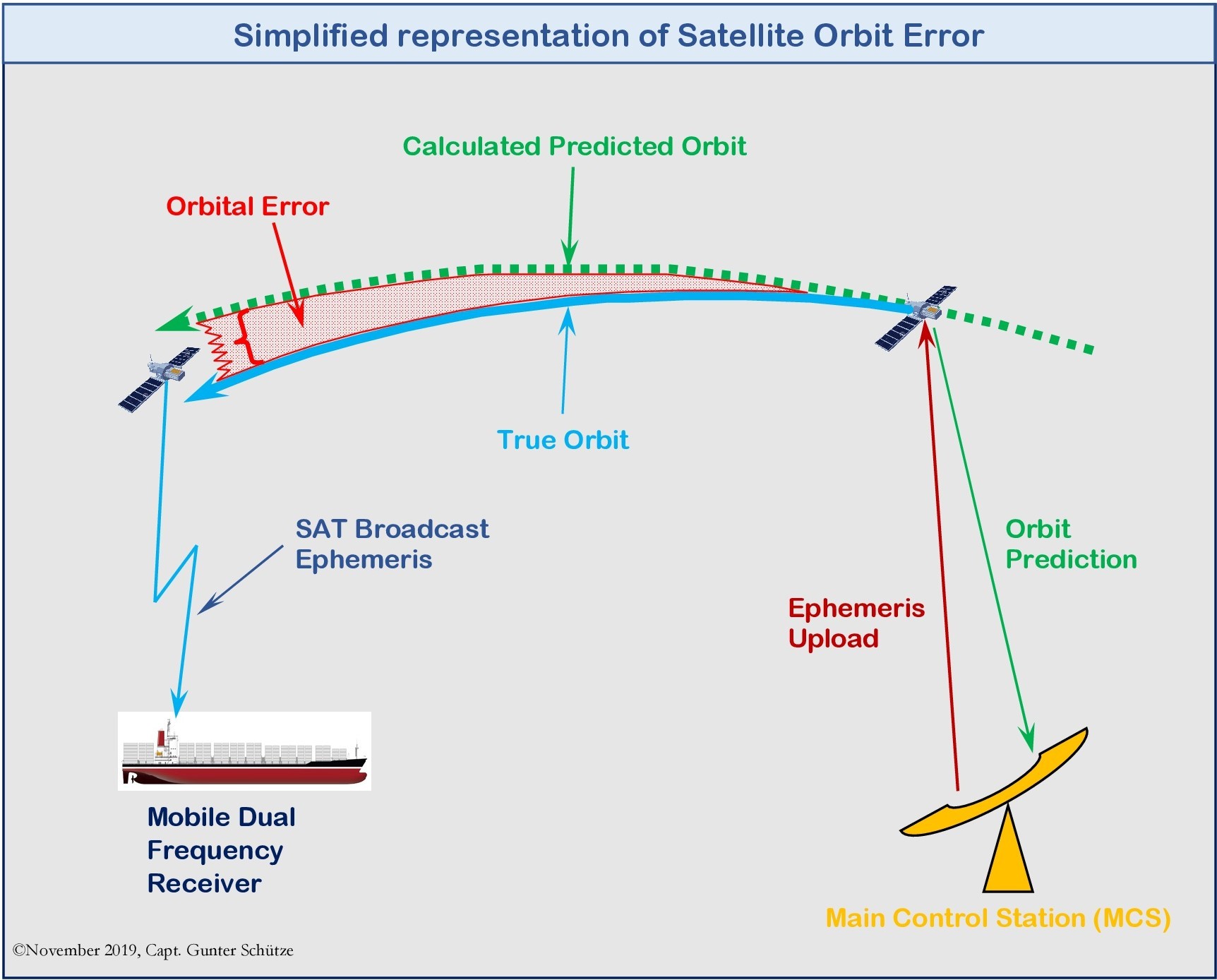
To calculate the position with GNSS, knowledge of the exact satellite position is required. The satellite positions contained in the GNSS navigation messages are predictions of where the satellite is likely to be located. Deviations between prediction and actual satellite position can have a probability of error of up to 10 meters. For the seafaring this value is relatively insignificant. But this looks in further kinds of use quit different, e.g. in geodesy
Causes of this error are:
The current position of a satellite is calculated from the transmitted ephemeris (precise orbit data) contained in the navigation messages. Ephemeris mathematically describes the predicted orbit of a satellite, which allows a receiver to determine the current position of a satellite in space at a given time. However, there are slight disturbances of the satellite orbit. These disorders can have different causes like:
These disorders can have different causes like:
a) the effect of the gravitational fields of the moon and the sun, whereby in particular the gravitational field of the moon has considerable influence,
b) the radiation pressure exerted by the sun on the satellites,
c) the movements of the satellites are affected by frictional forces from the rest of the atmosphere.
Consequence: the satellites are not exactly on the theoretically calculated orbit, as represented in the graphic for satellite orbit-error above, which in turn affects the position determination.
In order to keep the ephemerides always precise despite the disturbances that occur, the satellite orbits are permanently monitored by the GPS ground segment. As can be seen from the adjacent graphic using the example of GPS.
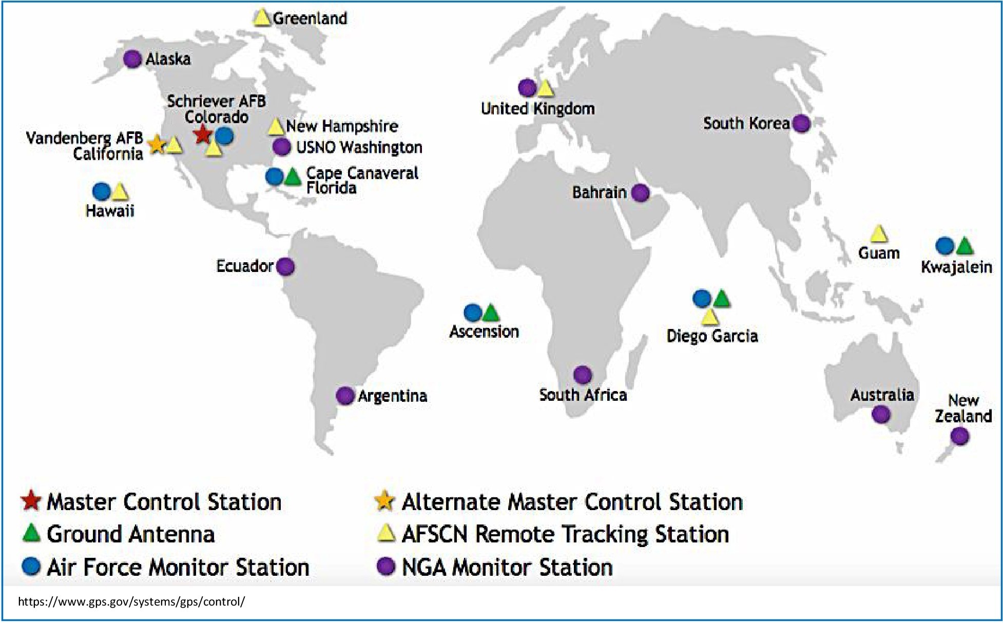
The data from the observations are used to calculate the orbit data in advance. The newly calculated orbit data is then transmitted to the satellites and updated hourly. To get even more accurate orbit data, the satellites are not only observed by the GPS ground segment, but also by a large number of worldwide distributed observation stations. These observation stations belong to the international GPS Service.
1.2. Clock error in the satellite
In GPS (Part 1), it was explained in the subject time dilation and gravitational dilation that even the slightest time deviation of the clocks in the receivers compared to the time in the clocks of the satellites can cause considerable position errors. However, the use of atomic clocks, because of their higher accuracy, does not protect them from interference. The time in the satellites is determined by the satellite atomic clocks. Nevertheless, there is a time difference between the satellite time and the GPS system time. The reason lies in the effects of dilatation. This happens partly because of the speed of a satellite, because the satellite clock is relatively slower than a non-moving clock on the earth's surface and partly because of the lower gravity field of the earth in the satellite orbit. As a result, a satellite clock is faster than a resting clock on the earth's surface (gravitational dilation). The clock error has an influence on the accuracy of the path data (ephemeris error) and thus also on the accuracy of the distance measurement. This is because the ephemeris are assigned to a wrong time.
The deviation of the satellite time from the GPS system time is determined for each satellite in the Main Control Station (MCS) and transmitted to the satellites using the ground transmitter station. The satellites then transmit the time correction parameters in the navigation message (in the so-called sub-frames of the navigation message).
1.3. Geometric Errors of Satellites - Dilution of Position (DOP)
The accuracy of positioning with satellites is highly dependent on the satellite geometry, that is, the distance angles between the satellites. It is called DILUTUON of POSITION (DOP) and stands for the influence of satellite geometry on the measurement accuracy. In other words - DOP - stands for the weakening of the position accuracy and is thus a measure of the satellite constellation-dependent inaccuracy.
The more acute the angles between the satellites observed, the less accurate the position determined. The background to this is that the intersections of the distance lines of corrected distance and pseudo-error removal result in large error areas in comparison to distance angles of > 30 °.
It follows the same principle, which is used in traditional navigation (terrestrial, radio navigation, astronomical) application that angles of <30 ° in their intersections in any case adversely affect the accuracy of positioning, since an accurate intersection assignment is only possible inaccurately , due to long cutting lines. They should therefore not be used.
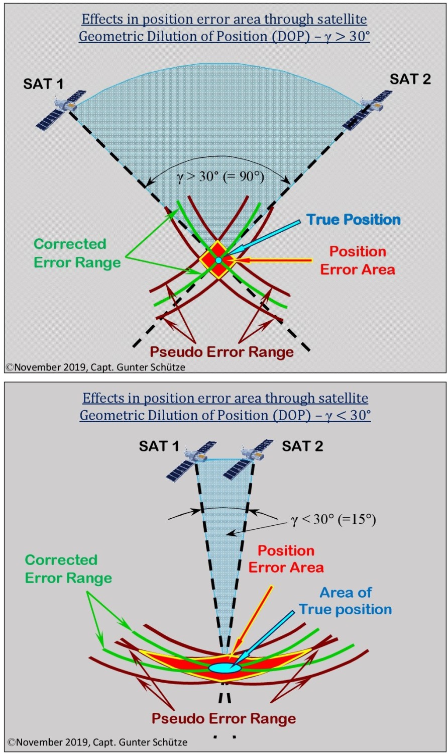
In the left-hand diagram, this is illustrated by an example with 2 satellites, with a distance angle γ > 30 ° and γ < 30 ° and the associated effects on the position accuracy and the area of the region of the position error.
Angles of γ > 30 ° (90 ° in the example), it can be seen that the dimension of the area of the region of the position error is significantly smaller and thus the position determined is significantly more accurate than with distances of γ < 30 ° (15 ° in the example). Where the area of the position error and thus also the region of the possible determined position increases significantly.
The logical conclusion is that if 4 satellites are used for observation and they are close to each other, i.e. with small distance angles, this means that the accuracy of the position determination is reduced. If the distance angles between these satellites are increased, this means that the accuracy of the position determination is increased. Optimum positioning accuracy is achieved when all 4 satellites are distributed at 120 ° intervals, with one satellite at the zenith of the receiver and the other 3 satellites should have a relatively small elevation above the horizon. However, too low elevation angles also mean a higher influence of atmospheric disturbances.
The last listed satellite constellation would mean that the DOP would take on the minimum value, so there are optimal conditions for determining the position.
From this it can be concluded that the larger the DOP value, the greater the expected inaccuracy in the position. In other words, the DOP value is proportional to the accuracy of the measurement.
Thus, when the DOP value doubles, the error value of the position determination also doubles.
In the specialist literature, it is formulated by the Swiss J. M. Zogg, in his publication "GPS and GNSS: Basics of positioning and navigation with satellites", published in 2015, as follows:
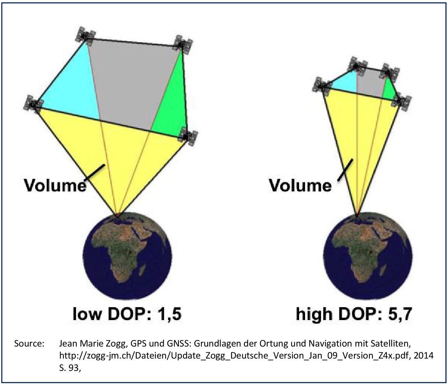
The DOP value "(...) can be interpreted as the reciprocal value of the volume of a tetrahedron formed from satellite and user positions" (p. 92).
When the volume of the tetrahedron reaches its maximum, the DOP value reaches its minimum (see figure above).
An illustrative example of how the DOP changes depending on the satellite constellation. DOP is therefore a variable value that must be considered in relation to the variability of the satellite configuration and is subject to constant change.
1.3.1. DOP values and their differences
DOPis divided into the following values:
a) GDOP: referred to as Geometric DOP. Value Describes the influence of satellite geometry and timekeeping on position in space (3D). For a good position determination, the GDOP value should be <5.
b) PDOP: referred to as Position DOP. The value Describes the influence of the satellite geometry on the 3D position
c) HDOP: referred to as Horizontal DOP. The value describes the influence of the satellite geometry on the position in the plane (2D). Meaning of accuracy values for HDOP: < 4 very good, 4 - 6, good, 6-8, inaccurate, > 8 not usable. The higher the selected satellites in the sky, the worse the HDOP values.
d) VDOP: referred to as Vertical DOP. Value Describes the influence of satellite geometry on altitude (1D). The VDOP values are bad as soon as the satellites are very close to the horizon.
e) TDOP: referred to as Time DOP. The value describes the influence of the satellite geometry on the time measurement
GDOP is the most important DOP value because it represents the error information of the entire system. It results from the position DOP (position error in space) and Time DOP (time offset) and is calculated as follows:

From this it becomes clear that the value GDOP is dependent on the location of the receiver and the time.
If more than 4 satellites on the visible horizon, the receiver selects the 4 satellites that give the best GDOP value and thus have the most favorable satellite constellation.
1.4. Satellite elevation effects on the VDOP
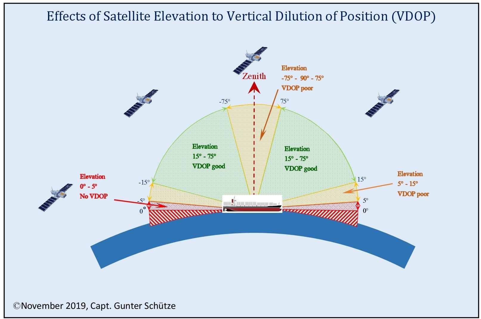
The adjacent graphic shows the influence of satellite elevation on VDOP quality. Again, the smaller the VDOP value, the better the satellite constellation.
An elevation between (-75 °) - Zenith (90 °) - (+ 75 °) and between 5 ° - 15 ° means less favorable VDOP values, which adversely affect the position determination. Particularly low-altitude satellites are more exposed to atmospheric disturbances because their signals travel a longer distance in the atmosphere, which causes a delay in the signal resulting in larger range finding errors.
Heights between 0 ° - 5 ° result a very large VDOP, which can no longer be used for position determination, since the influence of atmospheric disturbances becomes too great to receive a usable satellite signal for the distance measurement.
Under normal conditions, satellite elevations between 15 ° to 75 ° elevation are the most favorable angles for maritime GNSS receivers to limit rangefinding errors due to atmospheric disturbances. However, it is possible by manual adjustment to change the elevation angle to be used. Likewise, in the GNSS (GPS) configurations, the sub-menus of the receivers display the values for HDOP and VDOP, thus providing information about the quality of the satellite data and thus the accuracy of the distance measurement. Depending on the particular manufacturer of GNSS receivers, they are also referred to as Satellite angle or VDOP. Signal to Noise Ratio (SNR) describes the signal quality and is represented by various diagram shapes (bar graphs, line graphs).
In addition, the data used for the local DGPS beacons can be called up in order to obtain an overview of the signal quality and accuracy of the positioning of DGPS.
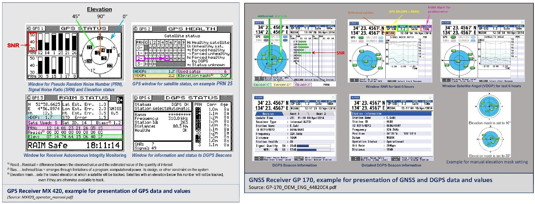
RAIM…Receiver Autonomus Integrity Monitoring- technology developed to assess the integrity of global positioning system (GPS) signals in a GPS receiver system. It is of special importance in safety-critical GPS applications, such as in aviation or marine navigation
SNR…Signal to Noise Ratio-- Measure of the technical quality of a useful signal, which is superimposed by a noise signal.
For detailed instructions on how to use and the settings of the GPS / GNSS receiver, refer to the Operational Manuals provided by the manufacturers.
2. Errors affecting signal propagation
Since we are dealing at satellite signals as electromagnetic waves, they are also subject to the laws of physics of the propagation of waves. Especially when waves enter media of different densities. This means that the physical principles of refraction and reflection come into play. On the way from the satellite to the receiver, the electromagnetic waves undergo three different media of different ionization and density, which influence the wave direction and the propagation velocity of the wave. Since satellites in GPS at a height of 20200 km have their orbit around the earth, we have to divide into 3 different spheres:
a) Interplanetary space (> 1000 km - ∞)
b) Ionosphere (60 - 1000 km)
i. Exosphere (700 - 1000)
ii. Thermosphere (85-700 km)
iii. Mesosphere (50-85 km)
c) Stratosphere 15-50 km
d) Troposphere 0-15 km
The stratosphere is not considered in the further analysis, as its effects on the satellite signals can be neglected.
In interplanetary space, due to its extremely low gas density, there is an almost unrestricted linear wave propagation with almost no friction losses, since it resembles a vacuum, a space void of air. The propagation speed electromagnetic / light waves takes place there at the speed of light.
That changes with the transition from the interplanetary space to the Ionosphere.
2.1. Basics of atmospheric effects
2.1.1 Ionospheric effects (at a height of 60 - 1000 km)
As the name implies, the ionosphere is an atmospheric layer containing large amounts of ions and free electrons. High-energy hard UV and X-rays of solar radiation cause ionization of the gas molecules.
The ionosphere plays a crucial role in radio communications due to their local layers with their ionization maximum. The ionization of these layers is influenced by the daily and seasonal course of the sun, as well as by the solar cycle (11 years). The ionization depends on the solar radiation intensity and the location. Why the dependence on the place? At the equator we find the strongest ionization during the day, which decreases towards the poles. The background is that in the equatorial region the atmosphere has its greatest extent.
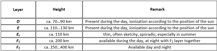
The factors mentioned have a significant influence on the character of the ground and space waves in the different frequency ranges of long / medium and short waves and can reach ranges of up to 1000 km in the best case. With overreach up to 2500 km are possible. The following table shows the structure of the 3 local layers and their sublayers of the ionosphere.
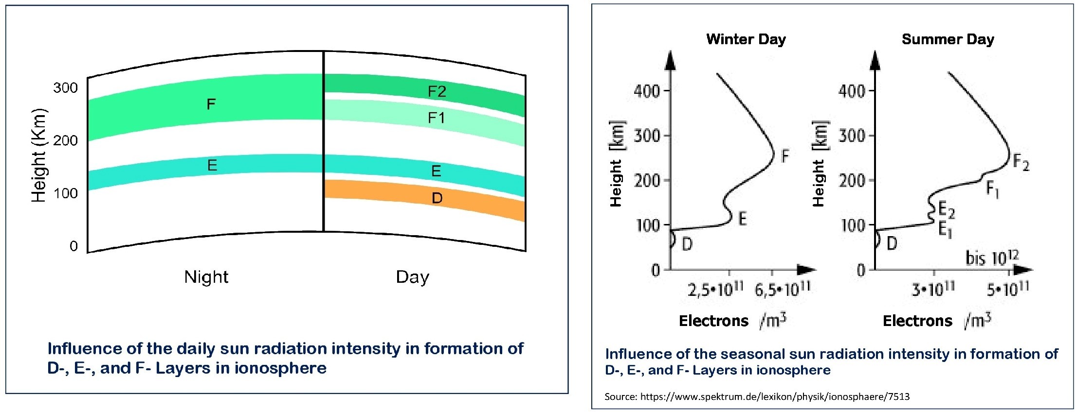
As mentioned, the structure of the ionized D-, E-, and F-layer is strongly dependent on the influence of the daily and seasonal sun-rise and the associated radiation intensity of the sun. How this is pictorially illustrated are shown in the two following graphics.
When the satellite signal enters the denser ionosphere from interplanetary space, two wave phenomena occur. The refraction and reflection of the wave.
2.2. Physical basics of wave propagation
As a short introduction to the understanding of wave propagation a short explanation of reflection and refraction
2.2.1. The Reflection
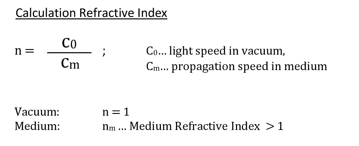
Reflection in physics means the reflection of waves on surfaces of different density (also called interfaces) depending on the characteristic impedance of the different media or the refractive index of the electromagnetic wave (called the propagation medium)
The energy of electromagnetic radiation is usually only partially reflected at an interface. Also referred to as partial reflection.
The basis of reflection is the law of reflection, which states that if the incident beam, the perpendicular, and the outgoing beam lie on one plane, then the angle of incidence α = the angle of departure α '.
The refractive index reflects the ratio of the wavelength of the light and thus the phase velocity in vacuum to another medium. In general it depends on the wavelength. That is, waves of different wavelengths can be reflected to different degrees.
The other part of the energy penetrates the 2nd layer and exits at the back side. Depending on the refractive index n, which is determined as follows
This results in the angle of refraction which results from the law of refraction.
2.2.2. The Refraction
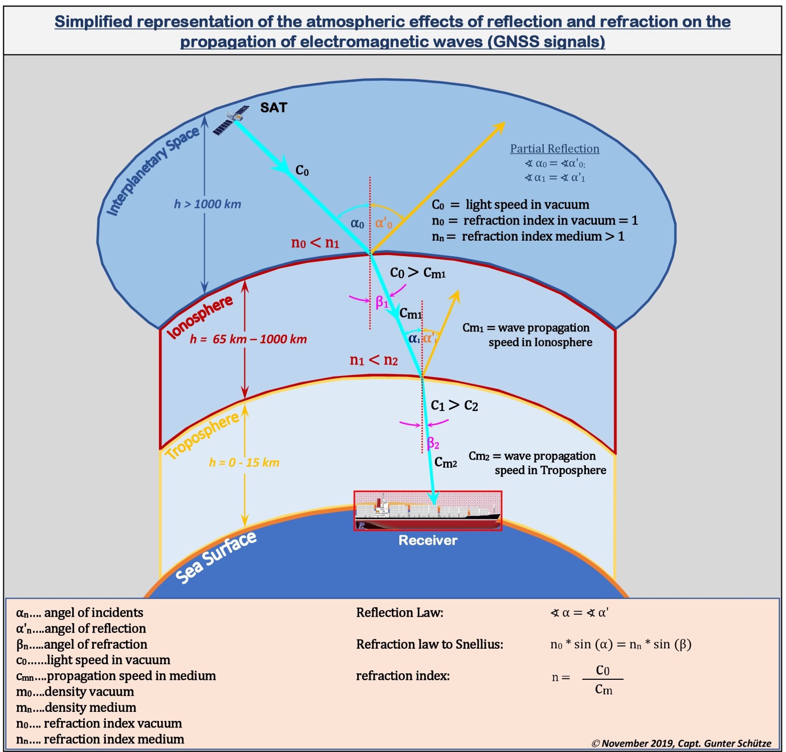
Refractionin physics means changing the propagation direction of waves through a spatial change in the refractive index of the medium which the wave passing through. The change in the refractive index leads to a change in the phase velocity (c) of the shaft. Refraction occurs with any type of waves that propagate in more than one dimension.
The basis of the refraction is the law of refraction by Snellius (Willebrord van Roijen Snell, 1580-1626, Dutch astronomer and mathematician).
It describes the change of direction of the direction of propagation of a plane wave during the transition to another medium. The cause of the change in direction is the change in the material-dependent phase velocity, which enters the refractive law as a refractive index. The most well-known phenomenon described by the law of refraction is the directional deflection of a light beam as it passes through a media boundary. The law is not limited to optical phenomena, but valid for any wave, especially ultrasonic waves.
In all the processes of reflection and refraction, it must be taken into account that this also involves energy losses, which cause the signal in the satellite signal to be reduced.
2.2.2. The Refraction
On the way from the satellite through the interplanetary space, the satellite signal propagates in a straight line and at the speed of light. Upon entry into the ionosphere, i.e. into the denser medium, caused by the ionization of the gases located there, by the sunlight, a part of the wave is reflected at the interface (partial reflection), while the other part of the wave is refracted at the interface and the dense medium passed through. Thereby it results in a propagation delay of the satellite signal, it will be attenuated, it slows down and there is a change in direction of the wave, caused by the change in the wavelength at penetration of the interface. The reduced propagation speed of the satellite signal causes a delay of the signal. This so-called ionospheric delay is frequency-dependent and can be up to 300 ns in the worst case, which would correspond to a position error of about 100 m. Since waves with high frequencies, i.e. in the L band (frequency range 1-2 GHz, λ = 30-15 cm), are exposed to the influences of the ionosphere less, it follows as a logical conclusion to use these for satellite navigation.
It thus becomes apparent that the sun plays a significant role in the effect of the ionospheric error as a deciding factor, which depends on the daily routine, the annual cycle of the sun and the solar cycles (11 years). It must be pointed out that the so-called twilight or night effect in the ionosphere (polarization changes of space waves), which occurs after the sunset (reduction of ionization in the ionosphere), can have effects on satellite signals. The ionosphere error is a frequency dependent error. This distinguishes him from the troposphere. He can be determined by using of two frequencies and eliminated up to 99%.
However, since only one frequency (GPS - L1) is available in the navigation for the public, this error must be reduced by means of geophysical calculation models. The best-known model is the Klobuchar model, named after its developer. It is based on the approximation of the vertical ionospheric transit time delay by a cosine function of the local time during the day and a constant magnitude for the night and compensates for about 50% of the error.
2.4. The Troposphere error
The troposphere as the lowest layer of the earth's atmosphere from the earth's surface to about 15 km in height is characterized by the fact that their density decreases with altitude. The main causes of the tropospheric error are satellite elevation angles, temperature, humidity and the density of the gas molecules. It can be put into simple terms: the higher the density and temperature, the lower the humidity in the troposphere and the smaller the satellite elevation angle, the greater the propagation delay of the satellite signal, by attenuation to the propagation velocity of the wave, this means she is reduced, there is thus a time lag of the signal and of course there is also the influence of the refraction and partial reflection of the wave, so the refraction and reflection at the interface. The troposphere is not frequency dependent. The resulting tropospheric error is approximately 5 - 25 m in the distance measurement. Can amount up to approx. 33 m in extreme cases be.
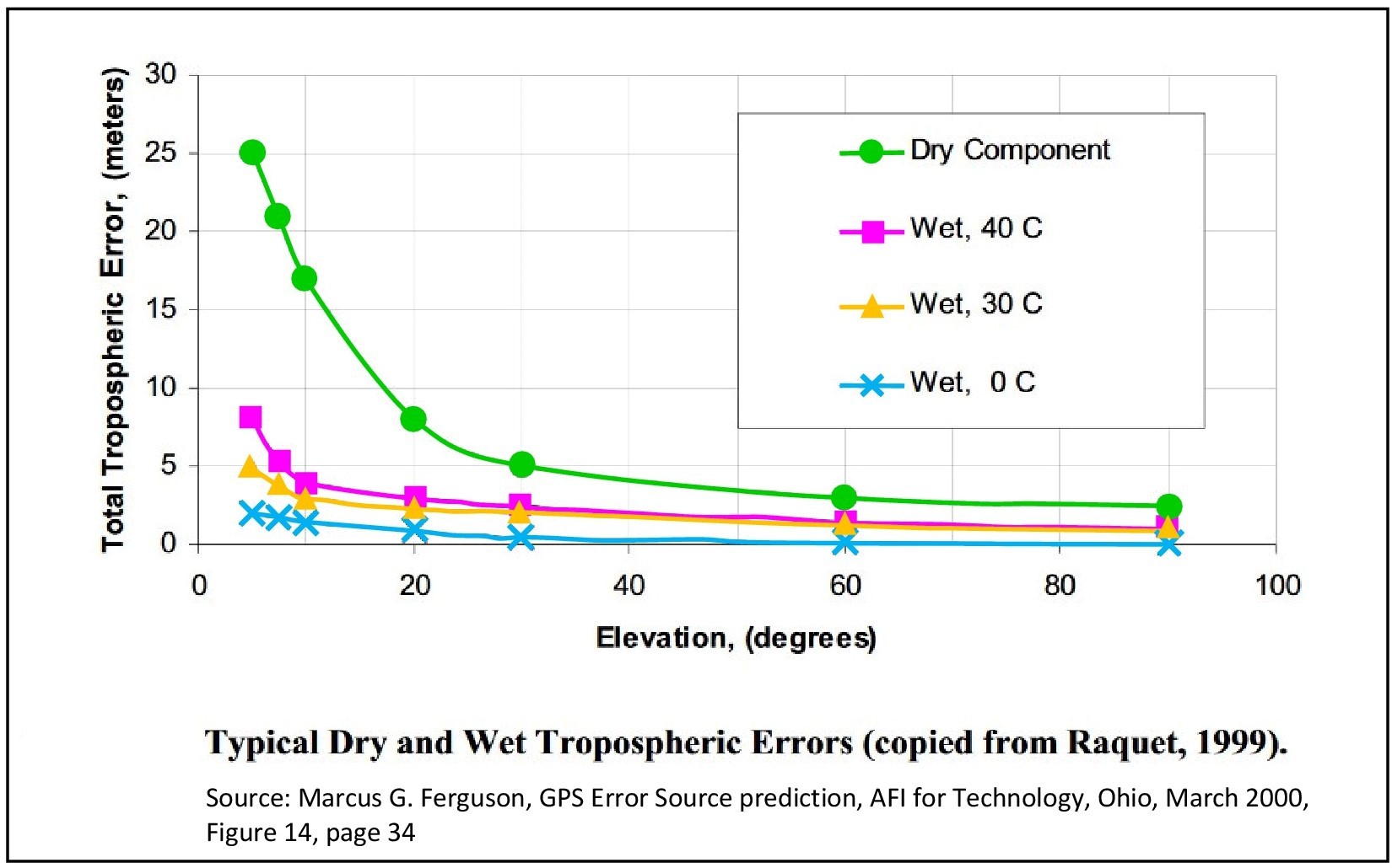
Tropospheric effects vary mainly due to the influence of the elevation angle of the satellites and the temperature of the region in which the receiver is located. Tropospheric models consist of a dry and moist component, whereby the dry component produces approx. 80 - 90% of the tropospheric error and the wet component approx. 10 - 20%, caused by the water vapor in the atmosphere. At an elevation angle of 90 °, the tropospheric error is predictable with an accuracy of up to 1% and in the best case close to 0. The graphic on the left illustrates the influence of satellite elevation, air humidity and air temperature on the tropospheric error. The tropospheric error has its least effects at satellite elevation angles > 15 ° and the greatest effects at angles of < 15 °, which results from the longer distance traveled in the troposphere and the associated time delays due to atmospheric influences. Whereas the dry component is very accurately predictable is this much more difficult with the wet component. Using algorithms installed in the receivers of existing models for dry and humid tropospheric conditions, so-called mapping functions (mapping functions are used to relate troposphere error at a particular elevation with troposphere error in zenith), it is possible the tropospheric error to almost compensate.
2.5. Receiver noise (Signal to Noise Ratio - SNR)
The signal-to-noise ratio is a measure of the technical quality of a useful signal, which is superimposed by a noise signal. It is defined as the ratio of the average power of the useful signal to the average noise power of the interference signal.
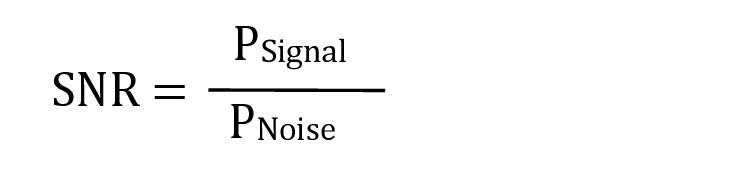
The formula is dimensionless
Both, signal and noise power must be measured at the same or equivalent points in a system and within the same system bandwidth.
To be able to extract the information safely from the signal, the useful signal must stand out clearly from the background noise, so the SNR must be sufficiently large. A ratio of more than 1: 1 (more than 0 dB) indicates more signal than noise.
As a characteristic value of a receiver, the SNR characterizes when the receiver can distinguish noise from the signal.
Using the definitions of SNR, signal and noise in decibels, this leads to an important formula for calculating the signal-to-noise ratio in decibels when the signal and noise are also in decibels.

I deliberately did not use the full logarithmic formula derivation because that would go beyond the scope and I can’t assume that in-depth knowledge of this technical area is available to the navigational officers on board. It's about basic understanding.
The receiver noise is primarily due to technical effects. And is different for the different reception systems:
We differentiate between 2 types of receiver noise:
a) Thermal noise
On the one hand, it can be traced back to receiver components. On the other hand, external conditions are reflected in the vicinity of the reception system.
b) Oscillator noise
It depends on the frequency standard used. A frequency standard is understood to be a frequency-stable oscillator. What atomic clocks are mostly used for today. The derived high-precision frequencies are referred to as normal frequencies.
The noise behavior of both components is also called white noise. The influences of the receiver noise are largely negligible due to the C / A code method used.
The consideration required in geodesy of the fluctuation of the phase center of the receiving antenna as a receiver error, for highly accurate surveying, is not important in maritime shipping
2.6. Multipath transmission / multipath propagation
These error factors only play a subordinate role in shipping on the open sea. They result from the refraction, diffraction, reflection and scattering of the satellite signals. They are interesting on canals, rivers and in port areas due to the physical effects mentioned for satellite signals on buildings, quay walls, steep bank walls, port crane systems.
3. Detection error
3.1. Receiver clock error
The distance between satellite and receiver is approx. 0.07 seconds taking into account the signal speed (speed of light with 299.792.458 m / s). With a required measuring accuracy of less than one meter, it requires watches with a very high accuracy of < 10-9 (ten to the minus 9). This is only possible with high-precision atomic clocks, which of course have their price. Taking into account economic constraints, watches with such accuracy are only installed in satellites. The receivers are equipped with less expensive, more temperature-stabilized atomic clocks, with a precision of 10-5 (10 to the minus 5) to 10-6 (10 to the minus 6). It can be seen that there is a measurement error that needs to be corrected by other means to achieve accuracies of less than one meter. In general, this is possible with algorithms that simulate the receiver clock error. Watch errors can be very diverse. In addition to constant and linear errors, there are also non-linear errors. Since material side measurements on the watch crystals would be very extensive and expensive, this problem must be clarified via software solutions. For this purpose, the clock error of the receiver at the time of determining the position is assumed to be constant. It is the same for all distance measurements. This means that if 4 satellites are measured, the clock error can be calculated as the fourth unknown. However, if other than the receiver clock error, other signal errors due to technical and physical errors at the receiver will occur, the method will fail. Then an increased mathematical effort is required to compensate for these errors.
3.2. Receiver electronics error
Errors in the receiver electronics cover a wide range of technical malfunctions:
Faulty fusess,
Antenna failure, faulty / corroded wire antenna connections and cable connections
Display problems,
Mainboard problems
Interface problems
Data port problems
LAN problems
Random Access Memory (RAM) error
Read-only memory (ROM) error
Ethernet problems (wrong / faulty IP address settings, faulty port settings and Ethernet errors, such as Check sum errors / syntax errors / framing errors etc.)
Failure of electronic components (transistors / circuits / CPU's / resistors / rectifiers)
It therefore makes sense to use the system intern tests integrated by the manufacturers in the receivers to detect internal errors in advance. In the Operational Manuals of the manufacturers, the necessary instructions and recommendations for action are given.3.3.
3.3. Error in the location of the phase center
This error is not relevant for aboard of ships GNSS receivers.
I want give it in a purely informative way to show that in surveying (geodesy), where high-precision position determinations of up to a few centimeters are used. The phase center of the receiving antennas used must be precisely adjusted, to fulfill the demand in very accurate positions.
3.4. Subjective factors
These are primarily human factors, i.e. incorrect or erroneous operations of the receiver by the user / operator, due to lack of or insufficient knowledge in the handling of the technique.
Especially when incorrectly entering important parameters [e.g. ship size and GNSS antenna positions, GNSS system assignment, elevation mask, RAIM alarm settings, reference date, I / O menu (data output sentence / TX interval / Ethernet - IP address / port) ECDIS synchronization- Configuration, etc.], errors of several hundred meters in the distance determination or malfunctions of the system until to complete breakdown can be triggered.
Final Remarks
As I wrote at the beginning, the ARTIFICIAL ERRORS listed under item 4 are dealt with separately in Part 3 for GPS. The background to this is that this chapter will in future become increasingly important in the mass use of GNSS in a wide variety of application areas.
That requires somewhat more intensive explanations in order to deal more intensively with the sometimes complicated subject matter and at the same time to point out that not everything that is sold to us sensationally in the media as jamming or spoofing, i.e. the targeted disruption by people, institutions, armed forces, governments, have something to do with it in real. Because there are also physical and technical causes for disturbances that can be significantly curbed by new technical solutions. For the user, this 4th chapter in part 3 of GPS should raise awareness, take a closer look at GNSS faults, analyze them with your possibilities, so also take a closer view at the surrounding area and derive correct conclusions.
Of course, this also presupposes that the knowledge gained in GPS Part 1 and Part 2 is applied correctly.
© Copyright December 2019, Capt. Gunter Schütze. Replication or redistribution in whole or in part is expressly prohibited without the prior written consent by Capt. M.Eng. Gunter Schütze
In the first part of my contribution about GPS, I wrote about the structure, the functionality, technical and physical basics of GPS:
To GPS (Part 1)
In my announced sequel, the second part of GPS, it is primarily about the technical and physical operational and functional limitations to which GPS is subject. These limitations, in part, have serious implications for the accuracy of GPS, and even go as far as limiting the functionality of GPS in its functions or even making it impossible. In doing so, I anticipate that these are errors that occur on a purely technical or physical basis. Much of these errors are taken into account in the configuration of GPS and implemented by means of appropriate correction tools, in GPS, so that unnoticed by the user, these errors are automatically corrected. But not all errors that occur can be solved by these tools. As a result, the GPS partially or temporarily limited in its functionality or temporarily even not effectively usable.
These bugs have nothing to do with SPOOFING/JAMMING. They are based on functional technical and physical causes, without human action. I will write more about spoofing/jamming at the following and last 3rd Part of GPS about artificial human initiated technical effects.
Let us therefore deal with the technical and physical sources of error that influence the function of GPS.
TYPES OF ERRORS
Below are several listed types of error, which of course should be the subject of closer consideration.
The division made by me relies on the corresponding error components.
It can also be distinguished into technical errors (see list under items 1, 3, 4) and natural errors (see item 2).
Priority will be given to errors which are highly relevant to satellite navigation in maritime shipping.
Some, rather untypical for the navigation GNSS errors are addressed only briefly. However, this is necessary as they are intended to help understand why in ports, in canals, in port approaches, GNSS data may be restricted in their accuracy and GNSS receivers limited in their function, until to temporary malfunctions.
Why is it important to know these types of errors?
All listed types of errors affect the operation and accuracy of GNSS. As can be seen, in this case GPS is not mentioned individually. Instead, the term GNSS (Global Navigation Satellite Systems) is used. The background is that all types of errors listed are applicable to all currently existing satellite navigation systems.
In the case of GPS-specific errors, this is of course only referred to GPS and marked.
1. Errors associated with satellites
1.1. Errors in the satellite orbit
1.2. Error in the satellite clock
1.3. Geometry of satellites
1.3.1. DOP values and their differences
1.4. Elevation errors
2. Errors affecting signal propagation
2.1. Basics of atmospheric effects
2.1.1. Ionospheric effects
2.2. Physical basics
2.2.1. The reflection
2.2.2. The refraction
2.3. Ionosphere error
2.4. Troposphere error
2.5. Noise of the receiver
2.6. Multipath transmission (reflection)
3. Recognition errors
3.1. Receiver clock error
3.2. Receiver electronics
3.3. Position of the phase center (refers primarily to the geodesic use)
3.4. Subjective factors
4. Artificial errors
4.1. Premeditated errors
4.2. Unintended Interferences
4.3. Intentional Interferences
4.3.1. Jamming,
4.3.2. Spoofing,
4.3.3. Meaconing
Item 4 with its sub-items is separately described by me in the 3rd part of GPS, due to its complexity and increasing importance in the civil and military use of GNSS
1. Errors associated with satellites
1.1. Errors in the satellite orbit
These errors, also called ephemeris errors, are based on the difference in the predicted satellite position and its actual position.
To calculate the position with GNSS, knowledge of the exact satellite position is required. The satellite positions contained in the GNSS navigation messages are predictions of where the satellite is likely to be located. Deviations between prediction and actual satellite position can have a probability of error of up to 10 meters. For the seafaring this value is relatively insignificant. But this looks in further kinds of use quit different, e.g. in geodesy
Causes of this error are:
The current position of a satellite is calculated from the transmitted ephemeris (precise orbit data) contained in the navigation messages. Ephemeris mathematically describes the predicted orbit of a satellite, which allows a receiver to determine the current position of a satellite in space at a given time. However, there are slight disturbances of the satellite orbit. These disorders can have different causes like:
These disorders can have different causes like:
a) the effect of the gravitational fields of the moon and the sun, whereby in particular the gravitational field of the moon has considerable influence,
b) the radiation pressure exerted by the sun on the satellites,
c) the movements of the satellites are affected by frictional forces from the rest of the atmosphere.
Consequence: the satellites are not exactly on the theoretically calculated orbit, as represented in the graphic for satellite orbit-error above, which in turn affects the position determination.
In order to keep the ephemerides always precise despite the disturbances that occur, the satellite orbits are permanently monitored by the GPS ground segment. As can be seen from the adjacent graphic using the example of GPS.
The data from the observations are used to calculate the orbit data in advance. The newly calculated orbit data is then transmitted to the satellites and updated hourly. To get even more accurate orbit data, the satellites are not only observed by the GPS ground segment, but also by a large number of worldwide distributed observation stations. These observation stations belong to the international GPS Service.
1.2. Clock error in the satellite
In GPS (Part 1), it was explained in the subject time dilation and gravitational dilation that even the slightest time deviation of the clocks in the receivers compared to the time in the clocks of the satellites can cause considerable position errors. However, the use of atomic clocks, because of their higher accuracy, does not protect them from interference. The time in the satellites is determined by the satellite atomic clocks. Nevertheless, there is a time difference between the satellite time and the GPS system time. The reason lies in the effects of dilatation. This happens partly because of the speed of a satellite, because the satellite clock is relatively slower than a non-moving clock on the earth's surface and partly because of the lower gravity field of the earth in the satellite orbit. As a result, a satellite clock is faster than a resting clock on the earth's surface (gravitational dilation). The clock error has an influence on the accuracy of the path data (ephemeris error) and thus also on the accuracy of the distance measurement. This is because the ephemeris are assigned to a wrong time.
The deviation of the satellite time from the GPS system time is determined for each satellite in the Main Control Station (MCS) and transmitted to the satellites using the ground transmitter station. The satellites then transmit the time correction parameters in the navigation message (in the so-called sub-frames of the navigation message).
1.3. Geometric Errors of Satellites - Dilution of Position (DOP)
The accuracy of positioning with satellites is highly dependent on the satellite geometry, that is, the distance angles between the satellites. It is called DILUTUON of POSITION (DOP) and stands for the influence of satellite geometry on the measurement accuracy. In other words - DOP - stands for the weakening of the position accuracy and is thus a measure of the satellite constellation-dependent inaccuracy.
The more acute the angles between the satellites observed, the less accurate the position determined. The background to this is that the intersections of the distance lines of corrected distance and pseudo-error removal result in large error areas in comparison to distance angles of > 30 °.
It follows the same principle, which is used in traditional navigation (terrestrial, radio navigation, astronomical) application that angles of <30 ° in their intersections in any case adversely affect the accuracy of positioning, since an accurate intersection assignment is only possible inaccurately , due to long cutting lines. They should therefore not be used.
In the left-hand diagram, this is illustrated by an example with 2 satellites, with a distance angle γ > 30 ° and γ < 30 ° and the associated effects on the position accuracy and the area of the region of the position error.
Angles of γ > 30 ° (90 ° in the example), it can be seen that the dimension of the area of the region of the position error is significantly smaller and thus the position determined is significantly more accurate than with distances of γ < 30 ° (15 ° in the example). Where the area of the position error and thus also the region of the possible determined position increases significantly.
The logical conclusion is that if 4 satellites are used for observation and they are close to each other, i.e. with small distance angles, this means that the accuracy of the position determination is reduced. If the distance angles between these satellites are increased, this means that the accuracy of the position determination is increased. Optimum positioning accuracy is achieved when all 4 satellites are distributed at 120 ° intervals, with one satellite at the zenith of the receiver and the other 3 satellites should have a relatively small elevation above the horizon. However, too low elevation angles also mean a higher influence of atmospheric disturbances.
The last listed satellite constellation would mean that the DOP would take on the minimum value, so there are optimal conditions for determining the position.
From this it can be concluded that the larger the DOP value, the greater the expected inaccuracy in the position. In other words, the DOP value is proportional to the accuracy of the measurement.
Thus, when the DOP value doubles, the error value of the position determination also doubles.
In the specialist literature, it is formulated by the Swiss J. M. Zogg, in his publication "GPS and GNSS: Basics of positioning and navigation with satellites", published in 2015, as follows:
The DOP value "(...) can be interpreted as the reciprocal value of the volume of a tetrahedron formed from satellite and user positions" (p. 92).
When the volume of the tetrahedron reaches its maximum, the DOP value reaches its minimum (see figure above).
An illustrative example of how the DOP changes depending on the satellite constellation. DOP is therefore a variable value that must be considered in relation to the variability of the satellite configuration and is subject to constant change.
1.3.1. DOP values and their differences
DOPis divided into the following values:
a) GDOP: referred to as Geometric DOP. Value Describes the influence of satellite geometry and timekeeping on position in space (3D). For a good position determination, the GDOP value should be <5.
b) PDOP: referred to as Position DOP. The value Describes the influence of the satellite geometry on the 3D position
c) HDOP: referred to as Horizontal DOP. The value describes the influence of the satellite geometry on the position in the plane (2D). Meaning of accuracy values for HDOP: < 4 very good, 4 - 6, good, 6-8, inaccurate, > 8 not usable. The higher the selected satellites in the sky, the worse the HDOP values.
d) VDOP: referred to as Vertical DOP. Value Describes the influence of satellite geometry on altitude (1D). The VDOP values are bad as soon as the satellites are very close to the horizon.
e) TDOP: referred to as Time DOP. The value describes the influence of the satellite geometry on the time measurement
GDOP is the most important DOP value because it represents the error information of the entire system. It results from the position DOP (position error in space) and Time DOP (time offset) and is calculated as follows:
From this it becomes clear that the value GDOP is dependent on the location of the receiver and the time.
If more than 4 satellites on the visible horizon, the receiver selects the 4 satellites that give the best GDOP value and thus have the most favorable satellite constellation.
1.4. Satellite elevation effects on the VDOP
The adjacent graphic shows the influence of satellite elevation on VDOP quality. Again, the smaller the VDOP value, the better the satellite constellation.
An elevation between (-75 °) - Zenith (90 °) - (+ 75 °) and between 5 ° - 15 ° means less favorable VDOP values, which adversely affect the position determination. Particularly low-altitude satellites are more exposed to atmospheric disturbances because their signals travel a longer distance in the atmosphere, which causes a delay in the signal resulting in larger range finding errors.
Heights between 0 ° - 5 ° result a very large VDOP, which can no longer be used for position determination, since the influence of atmospheric disturbances becomes too great to receive a usable satellite signal for the distance measurement.
Under normal conditions, satellite elevations between 15 ° to 75 ° elevation are the most favorable angles for maritime GNSS receivers to limit rangefinding errors due to atmospheric disturbances. However, it is possible by manual adjustment to change the elevation angle to be used. Likewise, in the GNSS (GPS) configurations, the sub-menus of the receivers display the values for HDOP and VDOP, thus providing information about the quality of the satellite data and thus the accuracy of the distance measurement. Depending on the particular manufacturer of GNSS receivers, they are also referred to as Satellite angle or VDOP. Signal to Noise Ratio (SNR) describes the signal quality and is represented by various diagram shapes (bar graphs, line graphs).
In addition, the data used for the local DGPS beacons can be called up in order to obtain an overview of the signal quality and accuracy of the positioning of DGPS.
RAIM…Receiver Autonomus Integrity Monitoring- technology developed to assess the integrity of global positioning system (GPS) signals in a GPS receiver system. It is of special importance in safety-critical GPS applications, such as in aviation or marine navigation
SNR…Signal to Noise Ratio-- Measure of the technical quality of a useful signal, which is superimposed by a noise signal.
For detailed instructions on how to use and the settings of the GPS / GNSS receiver, refer to the Operational Manuals provided by the manufacturers.
2. Errors affecting signal propagation
Since we are dealing at satellite signals as electromagnetic waves, they are also subject to the laws of physics of the propagation of waves. Especially when waves enter media of different densities. This means that the physical principles of refraction and reflection come into play. On the way from the satellite to the receiver, the electromagnetic waves undergo three different media of different ionization and density, which influence the wave direction and the propagation velocity of the wave. Since satellites in GPS at a height of 20200 km have their orbit around the earth, we have to divide into 3 different spheres:
a) Interplanetary space (> 1000 km - ∞)
b) Ionosphere (60 - 1000 km)
i. Exosphere (700 - 1000)
ii. Thermosphere (85-700 km)
iii. Mesosphere (50-85 km)
c) Stratosphere 15-50 km
d) Troposphere 0-15 km
The stratosphere is not considered in the further analysis, as its effects on the satellite signals can be neglected.
In interplanetary space, due to its extremely low gas density, there is an almost unrestricted linear wave propagation with almost no friction losses, since it resembles a vacuum, a space void of air. The propagation speed electromagnetic / light waves takes place there at the speed of light.
That changes with the transition from the interplanetary space to the Ionosphere.
2.1. Basics of atmospheric effects
2.1.1 Ionospheric effects (at a height of 60 - 1000 km)
As the name implies, the ionosphere is an atmospheric layer containing large amounts of ions and free electrons. High-energy hard UV and X-rays of solar radiation cause ionization of the gas molecules.
The ionosphere plays a crucial role in radio communications due to their local layers with their ionization maximum. The ionization of these layers is influenced by the daily and seasonal course of the sun, as well as by the solar cycle (11 years). The ionization depends on the solar radiation intensity and the location. Why the dependence on the place? At the equator we find the strongest ionization during the day, which decreases towards the poles. The background is that in the equatorial region the atmosphere has its greatest extent.
The factors mentioned have a significant influence on the character of the ground and space waves in the different frequency ranges of long / medium and short waves and can reach ranges of up to 1000 km in the best case. With overreach up to 2500 km are possible. The following table shows the structure of the 3 local layers and their sublayers of the ionosphere.
As mentioned, the structure of the ionized D-, E-, and F-layer is strongly dependent on the influence of the daily and seasonal sun-rise and the associated radiation intensity of the sun. How this is pictorially illustrated are shown in the two following graphics.
When the satellite signal enters the denser ionosphere from interplanetary space, two wave phenomena occur. The refraction and reflection of the wave.
2.2. Physical basics of wave propagation
As a short introduction to the understanding of wave propagation a short explanation of reflection and refraction
2.2.1. The Reflection
Reflection in physics means the reflection of waves on surfaces of different density (also called interfaces) depending on the characteristic impedance of the different media or the refractive index of the electromagnetic wave (called the propagation medium)
The energy of electromagnetic radiation is usually only partially reflected at an interface. Also referred to as partial reflection.
The basis of reflection is the law of reflection, which states that if the incident beam, the perpendicular, and the outgoing beam lie on one plane, then the angle of incidence α = the angle of departure α '.
The refractive index reflects the ratio of the wavelength of the light and thus the phase velocity in vacuum to another medium. In general it depends on the wavelength. That is, waves of different wavelengths can be reflected to different degrees.
The other part of the energy penetrates the 2nd layer and exits at the back side. Depending on the refractive index n, which is determined as follows
This results in the angle of refraction which results from the law of refraction.
2.2.2. The Refraction
Refractionin physics means changing the propagation direction of waves through a spatial change in the refractive index of the medium which the wave passing through. The change in the refractive index leads to a change in the phase velocity (c) of the shaft. Refraction occurs with any type of waves that propagate in more than one dimension.
The basis of the refraction is the law of refraction by Snellius (Willebrord van Roijen Snell, 1580-1626, Dutch astronomer and mathematician).
It describes the change of direction of the direction of propagation of a plane wave during the transition to another medium. The cause of the change in direction is the change in the material-dependent phase velocity, which enters the refractive law as a refractive index. The most well-known phenomenon described by the law of refraction is the directional deflection of a light beam as it passes through a media boundary. The law is not limited to optical phenomena, but valid for any wave, especially ultrasonic waves.
In all the processes of reflection and refraction, it must be taken into account that this also involves energy losses, which cause the signal in the satellite signal to be reduced.
2.2.2. The Refraction
On the way from the satellite through the interplanetary space, the satellite signal propagates in a straight line and at the speed of light. Upon entry into the ionosphere, i.e. into the denser medium, caused by the ionization of the gases located there, by the sunlight, a part of the wave is reflected at the interface (partial reflection), while the other part of the wave is refracted at the interface and the dense medium passed through. Thereby it results in a propagation delay of the satellite signal, it will be attenuated, it slows down and there is a change in direction of the wave, caused by the change in the wavelength at penetration of the interface. The reduced propagation speed of the satellite signal causes a delay of the signal. This so-called ionospheric delay is frequency-dependent and can be up to 300 ns in the worst case, which would correspond to a position error of about 100 m. Since waves with high frequencies, i.e. in the L band (frequency range 1-2 GHz, λ = 30-15 cm), are exposed to the influences of the ionosphere less, it follows as a logical conclusion to use these for satellite navigation.
It thus becomes apparent that the sun plays a significant role in the effect of the ionospheric error as a deciding factor, which depends on the daily routine, the annual cycle of the sun and the solar cycles (11 years). It must be pointed out that the so-called twilight or night effect in the ionosphere (polarization changes of space waves), which occurs after the sunset (reduction of ionization in the ionosphere), can have effects on satellite signals. The ionosphere error is a frequency dependent error. This distinguishes him from the troposphere. He can be determined by using of two frequencies and eliminated up to 99%.
However, since only one frequency (GPS - L1) is available in the navigation for the public, this error must be reduced by means of geophysical calculation models. The best-known model is the Klobuchar model, named after its developer. It is based on the approximation of the vertical ionospheric transit time delay by a cosine function of the local time during the day and a constant magnitude for the night and compensates for about 50% of the error.
2.4. The Troposphere error
The troposphere as the lowest layer of the earth's atmosphere from the earth's surface to about 15 km in height is characterized by the fact that their density decreases with altitude. The main causes of the tropospheric error are satellite elevation angles, temperature, humidity and the density of the gas molecules. It can be put into simple terms: the higher the density and temperature, the lower the humidity in the troposphere and the smaller the satellite elevation angle, the greater the propagation delay of the satellite signal, by attenuation to the propagation velocity of the wave, this means she is reduced, there is thus a time lag of the signal and of course there is also the influence of the refraction and partial reflection of the wave, so the refraction and reflection at the interface. The troposphere is not frequency dependent. The resulting tropospheric error is approximately 5 - 25 m in the distance measurement. Can amount up to approx. 33 m in extreme cases be.
Tropospheric effects vary mainly due to the influence of the elevation angle of the satellites and the temperature of the region in which the receiver is located. Tropospheric models consist of a dry and moist component, whereby the dry component produces approx. 80 - 90% of the tropospheric error and the wet component approx. 10 - 20%, caused by the water vapor in the atmosphere. At an elevation angle of 90 °, the tropospheric error is predictable with an accuracy of up to 1% and in the best case close to 0. The graphic on the left illustrates the influence of satellite elevation, air humidity and air temperature on the tropospheric error. The tropospheric error has its least effects at satellite elevation angles > 15 ° and the greatest effects at angles of < 15 °, which results from the longer distance traveled in the troposphere and the associated time delays due to atmospheric influences. Whereas the dry component is very accurately predictable is this much more difficult with the wet component. Using algorithms installed in the receivers of existing models for dry and humid tropospheric conditions, so-called mapping functions (mapping functions are used to relate troposphere error at a particular elevation with troposphere error in zenith), it is possible the tropospheric error to almost compensate.
2.5. Receiver noise (Signal to Noise Ratio - SNR)
The signal-to-noise ratio is a measure of the technical quality of a useful signal, which is superimposed by a noise signal. It is defined as the ratio of the average power of the useful signal to the average noise power of the interference signal.
The formula is dimensionless
Both, signal and noise power must be measured at the same or equivalent points in a system and within the same system bandwidth.
To be able to extract the information safely from the signal, the useful signal must stand out clearly from the background noise, so the SNR must be sufficiently large. A ratio of more than 1: 1 (more than 0 dB) indicates more signal than noise.
As a characteristic value of a receiver, the SNR characterizes when the receiver can distinguish noise from the signal.
Using the definitions of SNR, signal and noise in decibels, this leads to an important formula for calculating the signal-to-noise ratio in decibels when the signal and noise are also in decibels.
I deliberately did not use the full logarithmic formula derivation because that would go beyond the scope and I can’t assume that in-depth knowledge of this technical area is available to the navigational officers on board. It's about basic understanding.
The receiver noise is primarily due to technical effects. And is different for the different reception systems:
We differentiate between 2 types of receiver noise:
a) Thermal noise
On the one hand, it can be traced back to receiver components. On the other hand, external conditions are reflected in the vicinity of the reception system.
b) Oscillator noise
It depends on the frequency standard used. A frequency standard is understood to be a frequency-stable oscillator. What atomic clocks are mostly used for today. The derived high-precision frequencies are referred to as normal frequencies.
The noise behavior of both components is also called white noise. The influences of the receiver noise are largely negligible due to the C / A code method used.
The consideration required in geodesy of the fluctuation of the phase center of the receiving antenna as a receiver error, for highly accurate surveying, is not important in maritime shipping
2.6. Multipath transmission / multipath propagation
These error factors only play a subordinate role in shipping on the open sea. They result from the refraction, diffraction, reflection and scattering of the satellite signals. They are interesting on canals, rivers and in port areas due to the physical effects mentioned for satellite signals on buildings, quay walls, steep bank walls, port crane systems.
3. Detection error
3.1. Receiver clock error
The distance between satellite and receiver is approx. 0.07 seconds taking into account the signal speed (speed of light with 299.792.458 m / s). With a required measuring accuracy of less than one meter, it requires watches with a very high accuracy of < 10-9 (ten to the minus 9). This is only possible with high-precision atomic clocks, which of course have their price. Taking into account economic constraints, watches with such accuracy are only installed in satellites. The receivers are equipped with less expensive, more temperature-stabilized atomic clocks, with a precision of 10-5 (10 to the minus 5) to 10-6 (10 to the minus 6). It can be seen that there is a measurement error that needs to be corrected by other means to achieve accuracies of less than one meter. In general, this is possible with algorithms that simulate the receiver clock error. Watch errors can be very diverse. In addition to constant and linear errors, there are also non-linear errors. Since material side measurements on the watch crystals would be very extensive and expensive, this problem must be clarified via software solutions. For this purpose, the clock error of the receiver at the time of determining the position is assumed to be constant. It is the same for all distance measurements. This means that if 4 satellites are measured, the clock error can be calculated as the fourth unknown. However, if other than the receiver clock error, other signal errors due to technical and physical errors at the receiver will occur, the method will fail. Then an increased mathematical effort is required to compensate for these errors.
3.2. Receiver electronics error
Errors in the receiver electronics cover a wide range of technical malfunctions:
Faulty fusess,
Antenna failure, faulty / corroded wire antenna connections and cable connections
Display problems,
Mainboard problems
Interface problems
Data port problems
LAN problems
Random Access Memory (RAM) error
Read-only memory (ROM) error
Ethernet problems (wrong / faulty IP address settings, faulty port settings and Ethernet errors, such as Check sum errors / syntax errors / framing errors etc.)
Failure of electronic components (transistors / circuits / CPU's / resistors / rectifiers)
It therefore makes sense to use the system intern tests integrated by the manufacturers in the receivers to detect internal errors in advance. In the Operational Manuals of the manufacturers, the necessary instructions and recommendations for action are given.3.3.
3.3. Error in the location of the phase center
This error is not relevant for aboard of ships GNSS receivers.
I want give it in a purely informative way to show that in surveying (geodesy), where high-precision position determinations of up to a few centimeters are used. The phase center of the receiving antennas used must be precisely adjusted, to fulfill the demand in very accurate positions.
3.4. Subjective factors
These are primarily human factors, i.e. incorrect or erroneous operations of the receiver by the user / operator, due to lack of or insufficient knowledge in the handling of the technique.
Especially when incorrectly entering important parameters [e.g. ship size and GNSS antenna positions, GNSS system assignment, elevation mask, RAIM alarm settings, reference date, I / O menu (data output sentence / TX interval / Ethernet - IP address / port) ECDIS synchronization- Configuration, etc.], errors of several hundred meters in the distance determination or malfunctions of the system until to complete breakdown can be triggered.
Final Remarks
As I wrote at the beginning, the ARTIFICIAL ERRORS listed under item 4 are dealt with separately in Part 3 for GPS. The background to this is that this chapter will in future become increasingly important in the mass use of GNSS in a wide variety of application areas.
That requires somewhat more intensive explanations in order to deal more intensively with the sometimes complicated subject matter and at the same time to point out that not everything that is sold to us sensationally in the media as jamming or spoofing, i.e. the targeted disruption by people, institutions, armed forces, governments, have something to do with it in real. Because there are also physical and technical causes for disturbances that can be significantly curbed by new technical solutions. For the user, this 4th chapter in part 3 of GPS should raise awareness, take a closer look at GNSS faults, analyze them with your possibilities, so also take a closer view at the surrounding area and derive correct conclusions.
Of course, this also presupposes that the knowledge gained in GPS Part 1 and Part 2 is applied correctly.
© Copyright December 2019, Capt. Gunter Schütze. Replication or redistribution in whole or in part is expressly prohibited without the prior written consent by Capt. M.Eng. Gunter Schütze
 - Structure, mode of operation, technical and physical fundamentals of GPS")